Analysis Of McDonald's Menu Using Google Sheet
A former healthcare professional transitioning into Data Analytics.
Introduction
Hello all,
I am Namrata Joshi, a Physical Therapist and a NASM Certified Nutrition Coach. I am advancing towards a career change and learning Excel as a part of my journey. I wanted to combine my nutrition knowledge and Excel learnings and hence decided to use this dataset of Nutrition Facts for McDonald's Menu to analyze the data and create a useful dashboard. Any feedback and comments are welcomed and appreciated.
TL;DR
In this analysis, I have found the unique categories of items, menu items with the most proteins and beverages/tea & coffee/ smoothies & shakes low-calorie items with nutrition benefits.
I have used multiple Filters, Sort, Conditional Formatting, and UNIQUE, COUNTIF, SMALL and LARGE functions using various conditions to get to the specific data. I have also inserted different charts to my filtered and sorted data to represent the analysis visually.
The complete analysis can be found in this Google sheet.
Data Analysis
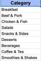
Finding unique menu categories.
I created a copy of the menu in a new sheet and named it menu_dataset. I further applied some formats in the first heading row to get a better read of the data.
Steps
Creation of
distribution of categoriessheetUse of a
UNIQUEfunction
=UNIQUE(menu_dataset!A:A)
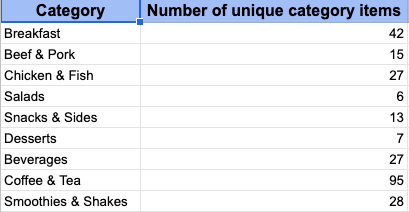
Finding the number of items in each category.
Steps
- I used a
COUNTIFfunction in the second column B.
=COUNTIF(menu_dataset!A:A, ""&A1)
- I used an autofill to copy the formula to the other cells in column B.
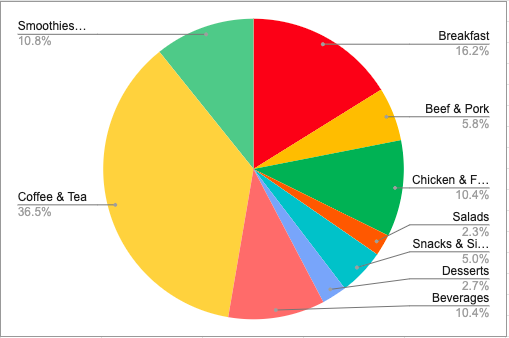
- Created a pie chart of unique categories and % of items in them.
Finding the high protein items.
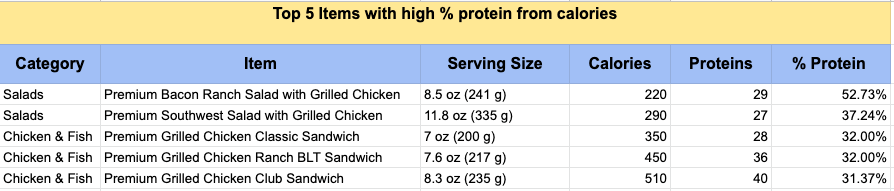
I found the items containing proteins>25 (the approximate amount recommended per meal for muscle protein synthesis). I later calculated % proteins( % of proteins from total calories in an item) and further retrieved a list of the top 5 items with high % protein.
Steps
Creation of
Items with high % proteinsheet.Finding items with protein>25.
I used the following filter function by selecting a range including categories, items, serving size and calories in menu_dataset sheet with a condition of protein>25.
=FILTER(menu_dataset!A2:D261,menu_dataset!T2:T261>25)
I also used the following filter function in a new column by selecting the range of the protein column in menu_datasetsheet with a condition of protein>25.
=FILTER(menu_dataset!T2:T261,menu_dataset!T2:T261>25)
- Creation of a new column (F)-
% protein.
I found out the % of proteins from the total calories of items. It was achieved by getting the total protein calories in an item first (Each gram of protein contains 4 calories) and then dividing it by the total calories of an item.
Hence, I created a new column and used the following formula by multiplying proteins column values by 4 and dividing by calories column values.
=(E2*4)/D2
I used an autofill to copy the formula for the other cells in column F.
- Inserting a note in the heading cell. I inserted the following note in the heading cell- % Protein (F1).

- Highlighting the top 5 items with high % protein. I used conditional formatting and the following LARGE function to achieve that.
=$F2>=LARGE($F$2:$F$38,5)
In the conditional format rule, I selected the range A2:F38 and used format cells if the custom formula is the above function. In this, LARGE function applies conditional formatting to test each row if it is larger than or equal to the 5th largest value. I later custom formatted the style filling the output values with light green 1 colour.
- Sorting the top 5 % Protein items.
I used the following SORTN function where I selected the range($A$2:$F$38)first and selected 5(as the number of results I want), 0 (as only five results to return), 6 (as the nth column to sort), and FALSE (to sort in descending order).
=SORTN($A$2:$F$38,5,0,6,FALSE)
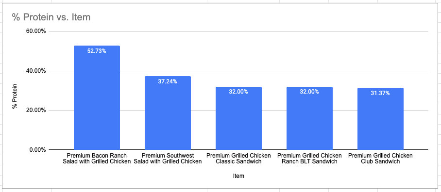
- Creating a chart listing items from highest to lowest % protein. I created a bar graph chart containing the top 5 items having the highest to lowest % protein values
Making healthier choices in menu drinks.
Steps
Creating a sheet named
Beverages, Tea/Coffee, Smoothies/Shakes.Finding items meeting their daily recommended values for saturated fats, cholesterol and total sugars.
I tried to find the items in the above categories meeting their daily recommended values for saturated fats<10%, cholesterol< 300 and sugars< 50(Approximate recommended values for total sugars), having some proteins, vitamin A and calcium. For this, I used the following filter function selecting a range of different adjacent and non-adjacent columns meeting the above conditions.
=FILTER({menu_dataset!A112:A261,menu_dataset!B112:B261,menu_dataset!D112:D261,menu_dataset!G112:G261,menu_dataset!P112:P261,menu_dataset!T112:T261,menu_dataset!U112:U261,menu_dataset!W112:W261},menu_dataset!I112:I261<10,menu_dataset!K112:K261<300,menu_dataset!S112:S261<50,menu_dataset!T112:T261<>0,menu_dataset!U112:U261<>0,menu_dataset!W112:W261<>0)
- Finding top 5 less calorie items having nutrition benefits.
I used conditional formatting and the following SMALL function to highlight the top 5 low-calorie items.
=$C2<=SMALL($C$2:$C$16,5)
In the conditional format rule, I selected the range A2:H16, used format cells if the custom formula is the above function. In the formula,SMALL function applies conditional formatting to test each row if it is smaller than or equal to the 5th smallest value. I later custom formatted the style filling the output values with light green 1 colour.
- Sorting 5 low-calorie items in their ascending order using the
SORTNfunction.
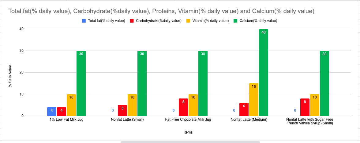
a) 5 low-calorie items with % daily value distribution.
This included sorting 5 low-calorie items and their % daily values of Total fat, carbohydrate, Vitamin A and Calcium using the following function.
=SORTN({$A$2:$E$16,$G$2:$H$16},5,0,3,TRUE)
I sorted a few columns with 2 different ranges containing the columns of category, Items, Calories, Total fat(% daily value), Carbohydrate(% daily value), Vitamin A(% daily value) and Calcium( % daily value). I later selected 5(as the number of results I want), 0 (as only 5 results to return), 3 (as the 3rd column of calories to sort), TRUE (to sort in ascending order).

- Bar graph chart
I hid the column of calories and inserted a bar graph chart selecting the columns of Items and (Total fats, carbohydrates, Vitamin A, Calcium) % daily values.
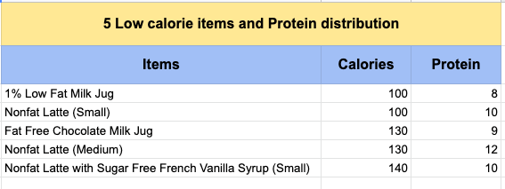
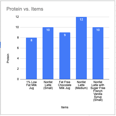
b) 5 low-calorie items with Protein distribution
This includes sorting 5 low-calorie items with their protein values using the following function.
=SORTN({$B$2:$C$16,$F$2:$F$16},5,0,2,TRUE)
I sorted a few columns with 2 different ranges containing the columns of Items, Calories and Protein. I later selected 5(as the number of results I want), 0 (as only 5 results to return), 2 (as the 2nd column of calories to sort), TRUE(sort in ascending order)
- Bar graph chart
I hid the column of Calories and inserted a bar graph chart selecting the columns of Items and Protein.
Lessons Learnt
I learnt effective ways to use the FILTER and SORT functions in this large dataset to get to the specific data.
I learnt a new way to select a range, especially for the non-adjacent columns which helped me to use the specific columns for the analysis.
I found the LARGE and SMALL functions very effective in the conditional formatting to highlight the rows meeting the specific conditions for a better visual representation of the data.
I learnt to customize my inserted charts to label the data in the Google sheet.